Evaluation of incident radiation by a V-Concentration System (VCS) in Bogotá, D.C.*

Evaluación de la radiación incidente por un sistema de concentración en V (SCV) en Bogotá, D.C.*

Avaliação da radiação incidente por um sistema de concentração V (VCS) em Bogotá, D.C. *

Carlos Augusto Bermúdez Figueroa ** 

 Carlos Eduardo Tibavisco Delgado ***

Universidad de Cundinamarca

Date Received: January 01 of 2018

Date of Acceptance: March 03 of 2018

Publication Date: April 01, 2018

DOI: http://dx.doi.org/10.22335/rlct.v10i4.600

* The article result of the investigation ". Evaluation of incident radiation by a V-Concentration System (VCS) in Bogotá, D.C." Universidad Cundinamarca.

** Master in Engineering with emphasis in Alternative Energies, Universidad Libre, and researcher at the University of Cundinamarca, Colombia. Affiliation: University of Cundinamarca. Email: carmetalbf@yahoo.es  Orcid: https://orcid.org/0000-0002-6132-8195

*** Specialist in Telematics from Los Andes University, and researcher at the University of Cundinamarca, Colombia. Affiliation: University of Cundinamarca. Email: ctibavisco@hotmail.com   Orcid: https://orcid.org/0000-0002-7496-4529

Abstract

The study presents the behavior of a V concentration system (VCS), as a way to estimate the incident radiation on a flat surface, based on the solar coordinates described in the equations of Spencer, J.W.

Increasing the areas of solar capture is a way to expand the solar radiation, captured on a flat surface by reflection. Maximizing the fraction of solar radiation captured; for that purpose, the V-Concentration System (VCS) was developed, adding four flat mirror surfaces to a flat surface, each with an inclination angle to the (flat) pickup surface. A statistical model was described to find a regression and thus expose the specific behavior areas of reflection on the (VCS), with the purpose of finding the optimal angle which achieves an increase in the uptake of radiation on a flat surface.

Keywords:  V-Concentration System (VCS), Incident Radiation, Flat Surface, Solar Radiation, Reflection.

Resumen

Se presenta un estudio para observar el comportamiento de un sistema de concentración en V (SCV), como medio para estimar la radiación incidente sobre una superficie plana, con base en las coordenadas solares descritas en las ecuaciones de Spencer, J. W.

Aumentar las áreas de captación solar es una forma para incrementar la radiación solar capturada por una superficie plana por medio de la reflexión. Maximizando la fracción de radicación solar captada; para tal propósito fue desarrollado el sistema de concentración en V (SCV), que agrega cuatro superficies de espejos planos a una superficie plana, cada una con un ángulo de inclinación respecto a la superficie de captación (plana). De estos se elaboró un modelo estadístico para encontrar una regresión y así exponer el comportamiento específico de las áreas de reflexión del (SCV), con el propósito de encontrar el ángulo óptimo que lograra un incremento en la captación de radiación sobre la superficie plana.

Palabras clave:  Sistema de concentración en V (SCV), Radiación incidente, Superficie plana, Radiación solar, Reflexión.

Resumo

Um estudo é apresentado para observar o comportamento de um sistema de concentração V (VCI), como um meio de estimar a radiação incidente em uma superfície plana, com base nas coordenadas solares descritas nas equações de Spencer, J. W.

Aumentar as áreas de captação solar é uma forma de aumentar a radiação solar captada por uma superfície plana por meio da reflexão. Maximizar a fração de radiação solar capturada; Para este propósito, foi desenvolvido o sistema de concentração em V (SCV), que adiciona quatro superfícies de espelhos planos a uma superfície plana, cada uma com um ângulo de inclinação em relação à superfície de coleta (plana). A partir deles, um modelo estatístico foi desenvolvido para encontrar uma regressão e, assim, expor o comportamento específico das áreas de reflexão (SCV), a fim de encontrar o ângulo ideal que alcançaria um aumento na captação de radiação na superfície plana.

Palavras-chave: V-Concentration System (SCV), Radiação incidente, Superfície plana, Radiação solar, Reflexão.

Introduction

The main propose of the present investigation is to show the behavior of a concentration system in V. At estimating the capture of incident radiation on a flat surface, thorough the reflection emitted by the inclined reflective surfaces (mirrors). The methodology used for the development of the research is shown in Figure 1.

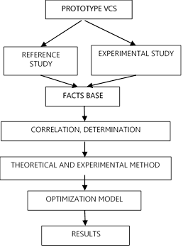
Figure 1. Research methodology.  Source: Authors.

First, the prototype of the V-concentration system was developed, which consists in adding four surfaces of flat mirrors to a flat collection surface, at different angles of inclination and a certain height, in order to collect experimental primary data.

Secondly, the mathematical calculation of reference was developed, with the objective of obtaining the average daily and annual global solar radiation of the system, based on mathematical methods provided by Spencer, JW and the information of governmental entities such as the Institute of Hydrology, Meteorology and Studies. Environmental IDEAM, and the Mining and Energy Planning Unit (UPME).

Subsequently, a statistical model was made, which achieved the best combination of the parameters that make up the V-concentration system, based on the results obtained from the theoretical and experimental calculation, the areas and angles of inclination of the reflective surfaces.

Finally, the behavior of the reference model was evaluated and the experimental one with the radiation obtained with the VCS.

Methodology 

VCS Prototype

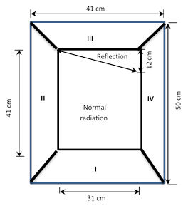
The prototype of the VCS consists in a flat surface and the four reflecting surfaces as illustrated in Figure 2, and in Figure 3, the prototype dimensions are shown. The aim of the prototype is to expand the areas of solar incidence on the reflecting surfaces; so by this mean the reflection on the flat surface would increase the solar uptake.

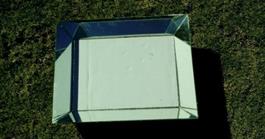
Figure 2. VCS prototype

Source: Authors.

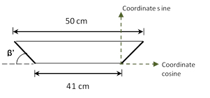
Figure 3a. VCS prototype dimensions

Source: Authors.

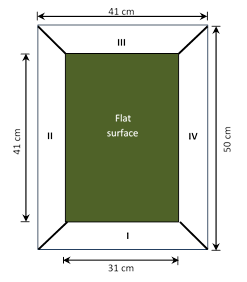
Figure 3b. VCS prototype dimensions

Source: Authors

Where:

I = Surface I

II = Surface II

III = Surface III

IV = Surface IV

β '= Angle by surface

Height reflective surfaces = 10 cm

Reference study

The objective of the reference study was to calculate the total daily H (B) radiation captured by VCS, based on the equations described by Spencer, in the solar Atlas, this information serves as a basis to correlate with the experimental data, and thus to be able to pose the model.

The objective of the reference study was to calculate the total daily H (B) radiation captured by VCS, based on the equations described by Spencer, in the solar Atlas, this information serves as a basis to correlate with the experimental data, and thus to be able to pose the model.

Experimental study

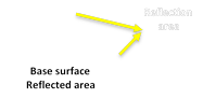
In days with direct irradiation in Bogotá, experimental data were taken. The prototype was placed to the south with a constant 5 ° inclination angle of the base surface in order to take samples and photographs, the reflecting surfaces with variable angles: 15 °, 30 °, 45 ° and 60 °, hour by hour in order to observe the behavior of the reflection, an example, is shown in Figure 4. It showed that the VCS forms different areas; areas of shadows, which indicate that the incidence of solar rays on reflecting surfaces is zero, areas of normal reflection, indicates that the incidence of solar rays is perpendicular to the flat surface, data that is not taken into account in the investigation and reflection areas that indicate the sun's rays affect the reflective surfaces and reflect on the flat surface; this was important data for the relevant database in the development of the model.

With the above information, the incident areas were graphed and marked on the flat surface, in order to obtain a total experimental H (β) radiation, the procedure was as follows: the fractions of shadow areas are calculated, and the areas of reflection, hour by hour, then the sum of the fractions of calculated areas is elaborated, with the reference H (β) obtained. Table 1 lists the results.

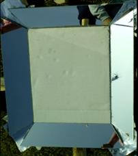
Figure 4. Reflection area at 8 am with angle 30 °

Source: Authors.

Table 1.

Global solar radiation of the system.

Source: Authors.

Table 2.

Areas and angles of each surface, and Calculation of sines and cosines of each of the angles.

Source: Authors.

Table 3.

Areas of reflection of the surfaces

Source: Authors.

In Table 1, it is exposed that the system presents a greater solar uptake when the angle of inclination of the four reflecting surfaces is 60 °, obtaining an H (β) of 4.336 kWh / m2 and 4.434 kWh / m2 which indicates an increase in global radiation compared to the reference value which corresponds to 3.57 kWh / m2 at 60 °. 

The areas of each surface with their respective angles of inclination with respect to the flat surface are shown (Table 2). The sine and cosine of the angles of each surface are calculated, data needed to realize the product of the areas with the sines and cosines in order to find the reflection areas of the surfaces with respect to the coordinates in cosine and sine, match in Table 3.

The database results from Table 3. From these, reflective areas, (cm²), in cosine and sine and the theoretical and experimental energy captured (kWh/m²), the correspondence between the variables and their relevance to the effect of the reflected area to propose a model.

Correlation coefficients.

The Pearson correlation coefficient (named after Karl Pearson, who formulated it) is a measure used in Statistics to calculate the degree of linear relationship between two random variables, therefore, it is also known as the linear correlation coefficient.

The correlation coefficients are determined by Excel. Among the following pairs of variables: the theoretical measure vs. the experimental, the theoretical measure vs each of the areas reflected in cosine and sine, as well as the experimental measure vs each of the areas reflected in cosine and sinus, with the purpose to quantify the proportion of resemblance (correlation) and explanatory (determination) between the pair of variables, as shown in the matrix of Table 4 and 5.

The data design leads to a multicollinearity situation which means that there is a strong correlation between each pair of variables mentioned above. For example, in Table 4, it is observed that the correlation coefficient between the theoretical and experimental measure is -0.66, which means that the experimental values ​​go in a direction opposite to the theoretical ones. When finding the coefficient of determination, for the same pair of variables, in Table 5, it is 44% that is to say that the behavior of the theoretical explains 44% of the experimental information, therefore, each one has an independent behavior 56%.

When comparing the correlations between the experimental measure vs the projected areas, from Table 4, it is identified that all have a value greater than 0.66, that is to say that all the surfaces have some contribution or decrease in the average value of the captured radiation measured experimentally, the above can be evidenced, so that all have a coefficient of determination higher than 44%, according to Table 5.

Table 4.

Correlation results

Source: Authors.

Table 5.

Determination results.

Source: Authors.

The correlation between the theoretical measure vs each one of the areas reflected in cosine and sine, of Table 4, is higher than 92% and this is reflected in the coefficients of determination above 85%, shown in Table 6, therefore, a high degree of correspondence is identified between the reflective areas of the theoretical and experimental studies. For this reason, a simple linear regression model is proposed.

Simple linear regression model.

•       = Daily average, (kWh/m²), of solar radiation based on the variable  

•       = coefficient, (kWh/m²), for the intercept of the data, based on the surface of the base.

•       = estimated coefficient, (kWh/m⁴), of the contribution per square meter, based on the projected surface.

•       X_i= fixed term or intercept, corresponding to the surface of the base or projected, m².

Formulation of the model.

For the construction of the specific model for the case studied, it was necessary to obtain the coefficients (B), that is a multiplicative factor, or constant number that is on the left of a variable or unknown, and multiplies it, in order to determine the energy captured by the VCS; by means of a statistical regression analysis in Excel, with a confidence interval of 95%, of the theoretical and experimental measure vs. the areas reflected in cosine and sine.

The summary of the models associated with the experimental data and the theoretical data found are shown in Tables 6 and 7. The first column contains the area or variable of which we are speaking, it is to remember that each area has a sine projection and another of cosine; the next column (r) is the correlation coefficient, indicates the similarity by projection; then the coefficient of determination follows (r^²); later there is the statistic (F) calculated in the regression; followed by stevedores of the model in the intercept and that of the variable.

The last two columns are associated with the probability of rejecting the coefficient of the intercept, the coefficient of the variable and the model. In this case, since there is only one independent variable, the P value of the model and the variable are the same.

In Table 6, it is observed that the correlation coefficients for the experimental data are not higher than 0.74, therefore, the adjusted r squared coefficients ​​are not greater than 0.47. However, in all cases the maximum permissible error level in the model is 0.051, that is, 5.1%.

For the theoretical data models, Table 7, there are correlation coefficients between 0.92 and 1.00. Which implies coefficients of determination between 0.83 and 1.00; all the F values ​​are greater than 40 and the significance of the intercept, models and variable in all cases have an error level lower than 0.001, that means, they are lower than one error in each 1000.

Therefore, it can be identified that the models provide information, through the respective coefficients of the daily energy average captured in kilowatts per hour for each surface in each of the cosine and sine components, thus with the previous coefficients it is possible have the information required to propose the optimization model.

Table 6.

Summary of models associated with experimental data.

Source: Authors.

Table 7.

Summary of models associated with the theoretical data.

Source: Authors.

Construction of the model

With the calculated coefficients we already have the information required to propose a linear statistical model for the case study, in order to evaluate the best combination of the parameters that make up the MCS, to find the increment of incident radiation on the surface flat

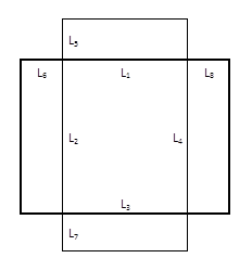
For its construction was used:

a) Structural design. Figure 5

b) Theoretical and experimental data base.

c) Objective function

d) Regression coefficients

e) Set of assumptions and restrictions.

The following model is formulated. Which is carried to a linear program of the VCS.

Figure 5. Variable system.   Source: Authors.

Objective function

Results

Mathematical models proposed

Reference model:

Table 8.

Theoretical captured radiation vs theoretical model

Radiation with theoretical model H(β)

Source: Authors.

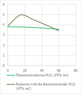
Figure 6.  Theoretical captured radiation vs theorical model. Source: Authors.

In Table 8 and Figure 6, the behavior of the reference model vs the theoretical radiation is shown, a very similar uptake between the different angles of inclination of the reflective surfaces can be observed, which indicates it is not relevant, so that the VCS theoretically would not work.

Experimental model:

Table 9.

Radiation captured experimental vs experimental model.

Source: Authors.

Figure 7. experimental captured radiation vs experimental model    Source: Authors.

In Table 9 and Figure 7, the behavior of the experimental model vs experimental radiation is shown, an increase in the uptake can be observed when the VCS presents a 60 ° inclination, which indicates that it is possible to adapt a flat panel to an VCS to increase solar gain.

Conclusions

The experimentally measured data show that the flat surface without VCS has a solar radiation catchment of 3.88 kWh / m2, when coupling the VCS at an angle of 60 ° with respect to the flat surface, it increases to 4.39 kWh / m2, equivalent to an additional 11.5% of catchment.

When checking the experimental model, it is observed that the flat surface without VCS has a solar radiation catchment of 3.77 kWh / m2, when coupling the VCS at an angle of 60 ° with respect to the flat surface, it increases to 4.63 kWh / m2, equivalent to an additional 18.5% of catchment.

Based on the above, it is shown that it is possible to increase the solar uptake by means of the reflection provided by the V-concentration system and to improve the use of incident solar radiation on the flat surface in Bogotá.

The results show that the solar uptake depends on the inclination angle of the system, the reflection areas involved in the flat surface, the angle of solar incidence and the climatic conditions of the site.

The mathematical model developed based on the experimental and theoretical study indicates that the V-concentration system can be adjusted to the physical conditions of a flat solar panel.

References

Banks, H. T.,  Shuhua Hu, W. Clayton Thompson-Modeling and Inverse Problems in the Presence of Uncertainty-Chapman and Hall_CRC (2014) (Monographs and Research Notes in Mathematics

Bione J. et al (2004). Comparison of the performance of PV water pumping systems driven by fixed, tracking and V-trough generators. Solar Energy 76 (2004) 703–711.

Canavos-Probabilidad y Estadistica - Aplicaciones y Metodos (Spanish Edition)-McGraw-Hill Companies (1994).pdf

Chechurin, V. L., Korovkin, N. V.  Hayakawa M. (auth.)-Inverse Problems in Electric Circuits and Electromagnetics-Springer US. Mathematical and Analytical Techniques with Applications to Engineering

Chong K.K. et al. (2012). Study of a solar water heater using stationary V-trough collector. Renewable Energy 39 (2012) 207-215.

Duffie, J. A., y Beckman, W. A. Solar Engineering of Thermal Processes. New York: John Wiley & Sons, 919p, 1991.

Frederick S. Hillier, Gerald J. Lieberman (late)-Introduction to Operations Research-McGraw-Hill Education (2015).pdf

Graham M. L. Gladwell, Antonino Morassi-Dynamical Inverse Problems_ Theory and Application (CISM International Centre for Mechanical Sciences.pdf

Hongfei Zheng et al. (2012) Experimental test of a novel multi-surface trough solar concentrator for air heating. Energy Conversion and Management 63 (2012) 123–129.

Nova, N., Pinzón, W., & Quinero, R. (2013). Hacia un nuevo modelo de cibernética, una aproximación al tercer orden. Bogota: Universidad Distrital.

Runsheng Tang y Xinyue Liu. (2011). Optical performance and design optimization of V-trough concentrators for photovoltaic applications. Solar Energy 85 (2011) 2154–2166.

Saffa Riffat y Abdulkarim Mayere. (2013). Performance evaluation of v-trough solar concentrator for water desalination applications. Applied Thermal Engineering 50 (2013) 234-244.

Sangani C.S. y Solanki C.S. (2007) Experimental evaluation of V-trough (2 suns) PV concentrator system using commercial PV modules. Solar Energy Materials& Solar Cells 91 (2007) 453–459.

Solanki C.S. et, al (2008). Enhanced heat dissipation of V-trough PV modules for better performance. Solar Energy Materials & Solar Cells 92 (2008) 1634–1638.

Spencer, J. W. Fourier Series Representation of the Position of the Sun. Search 2(5), 172p, 1971.

Tina G. M. y Scandura P.F. (2012). Case study of a grid connected with a battery photovoltaic system: V-trough concentration vs. single-axis tracking. Energy Conversion and Management xxx (2012) xxx–xxx.

UPME. Unidad de planeación Minero Energética. Atlas de Radiación Solar de Colombia. 2006. Apéndice A, B y C